Surface-wave breaking
The wave-breaking scenario has many similarities with the couette scenario: A shallow, non-rotating and unstratified water column is forced by a constant wind stress until the flow has become stationary. Now, however, near-surface turbulence generated by breaking surface waves is taken into acount as suggested by Craig and Banner (1994). In their approach, the injection of turbulence during the breaking process is modeled as a surface TKE flux that is proportional to the cube of the friction velocity. In this case, a so-called “transport layer” develops near the surface, in which TKE dissipation and vertical TKE transport balance, and all turbulence quantities follow power-law relationships. Data summarized in Umlauf and Burchard (2003) suggest, for example, that the TKE decays away from the surface with a power of approximately -2, whereas the turbulence length scale increases linearly with a slope close to L=0.2. As shown by Umlauf and Burchard (2003), this implies a linear decrease of the velocity profile. While all two-equation models investigated by Umlauf and Burchard (2003) do show a power-law decay of the TKE away from the surface, only their generic length scale (GLS) model reproduces the observed TKE decay rate of -2. Also the k-omega model with a predicted decay rate of -2.53 is approximately consistent with the observations, while the k-epsilon model fails (Umlauf et al., 2003). Below the transport layer, the solutions gradually converge to the classical law of the wall behavior of the couette scenario (logarithmic velocity profile, constant TKE, etc.).
The solutions for the k-omega models and the theoretical power-law relationships are shown in the figure below. After running GOTM for this scenario, you can reproduce the figure with the help of the plotting script plot_wave_breaking.py, which can also be found in the scenario directory. For this scenario, we also provide an alternative yaml file to run the GLS model for comparison. If you run GOTM with this input file, make sure to adjust the parameters and filename in plot_wave_breaking.py.
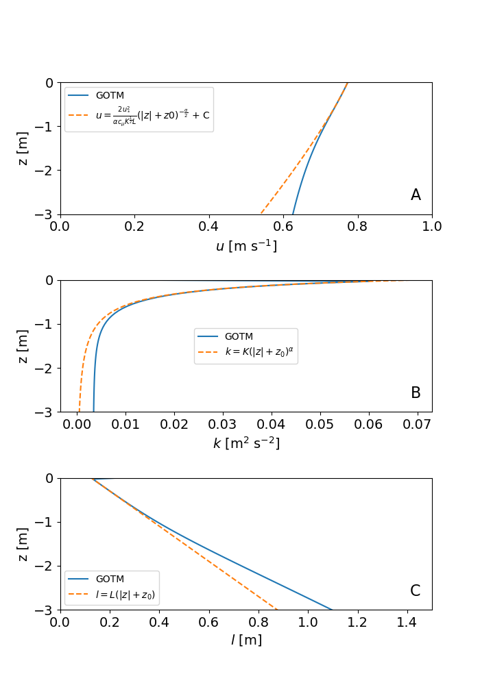
Profiles of (a) velocity, (b) turbulence kinetic energy, and (c) turbulence length scale (in red: theoretical power-law solutions). Results are shown for the k-omega model.