Surface- or bottom attached plume

In this idealised scenario, two types of plumes can be simulated: surface- and bottom attached plumes (density currents), driven by a sloping surface (interface between glacial ide and ocean water) or bottom.

Subglacial surface plume scenario:

The subglacial plume scenario described in a simple geometry the vertical structure of a subglacial plume rising under a sloping ice shelf - ocean interface. This scenario has been built by Burchard et al. (2022) to develop consistent ways of coupling melting processes at the ice-ocean interface with the turbulent stucture of the plume. This principle has also been applied by Reinert et al. (2023) for a two-dimensional study with vertical resolution and by Reinert et al. (2025) for a three-dimensional model of the 79 deg N glacier cavity.

The simulations analyzed here start from rest (zero velocity), with an initial plume thickness of D = 5 m. The ice-ocean interface is located at a depth of zb = −300 m and the water column is zb + H = 150 m deep, such that the bottom at z = −H = −450 m is sufficiently far below the ice to allow for an undisturbed plume deepening. This set of initial conditions allows for a subglacial plume that is quickly adjusted dynamically to the local conditions. The vertical discretization uses kmax = 500 layers with zooming toward the ice-ocean interface such that the resolution is gradually increasing from 0.5 m at the botttom to 0.09 m at the surface.

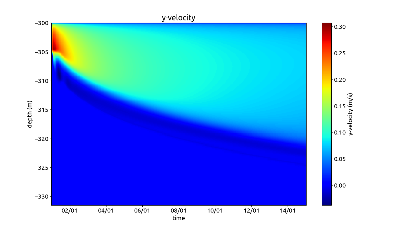
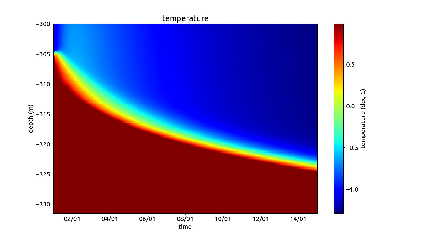
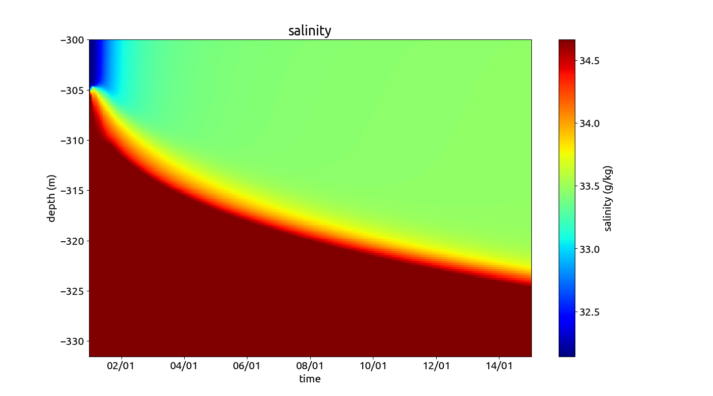
The ambient water is at rest and has a high ocean salinity of 34.5 g/kg and potential temperatures of 1°C. The initial plume salinity and potential temperature are 32 g/kg and −1°C, such that its potential density is lower than the potential density of the plume water. With this, the initial pressure gradient drives a subglacial plume rising upwards along the slope of the ice-ocean interface. The latitude of the water column location is 79 deg N, such that the Coriolis parameter has a value of f = 1.43 X 10^−4 1/s. The ice-ocean interface is sloping toward the north, while the slope toward the east vanishes. During the simulation time of 14 days, the plume velocity is expected to point toward the north-east direction as a consequence of the force balance between northward pressure gradient force, Coriolis force and frictional effects. The plume is subject to cooling and freshening due to melt fluxes at the ice-ocean interface and to warming and salinification due to entrainment of warmer and saltier ambient water. This simulation can be thought of as a plume underneath an infinite plain, where all plume properties are homogeneous along the interfacial slope.

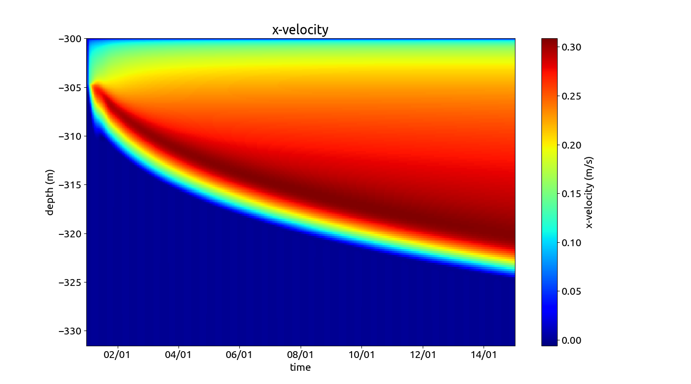
Bottom-attached plume scenario:

This scenario is motivated by medium-intensity gravity currents flowing into the Baltic Sea through the channel north of Kriegers Flak (55 deg 08’ N, 13 deg E) in the Western Baltic Sea, as observed and simulated using GOTM by Arneborg et al. (2007).

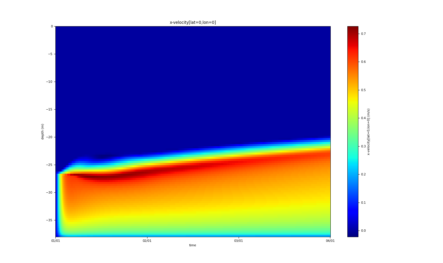
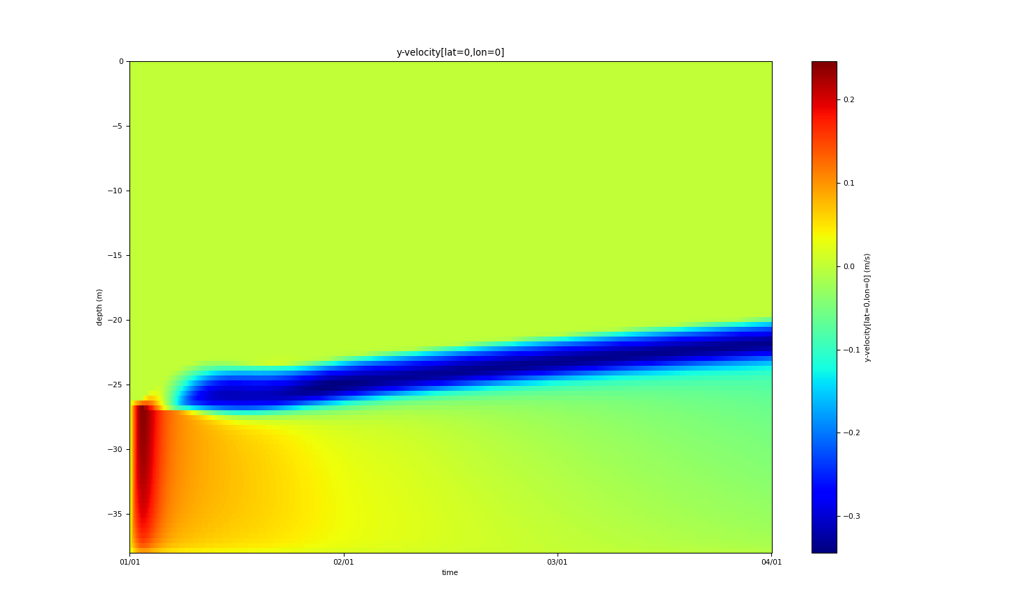
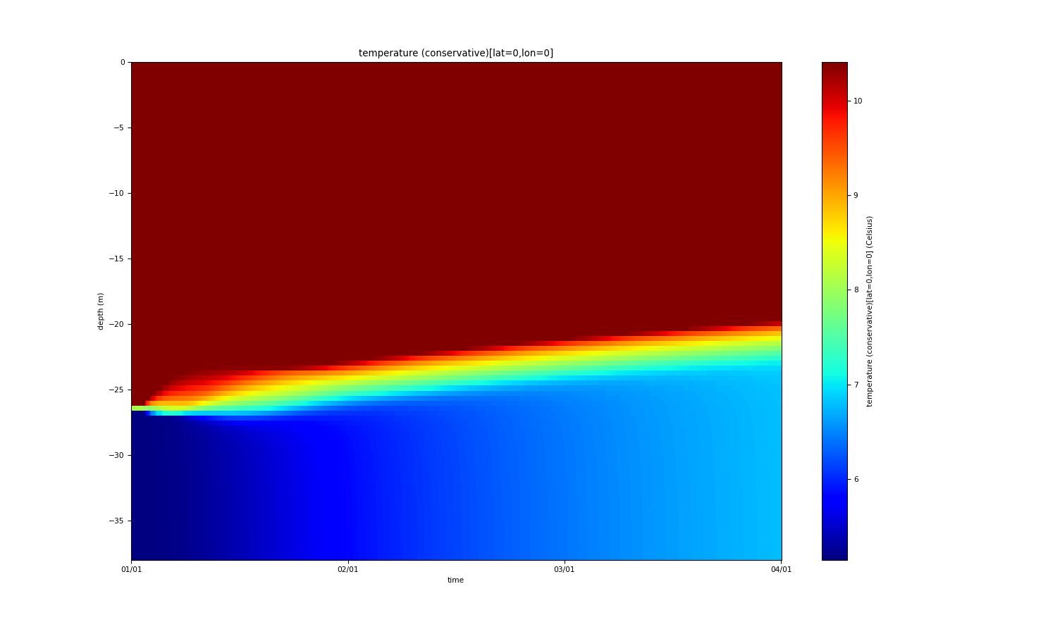
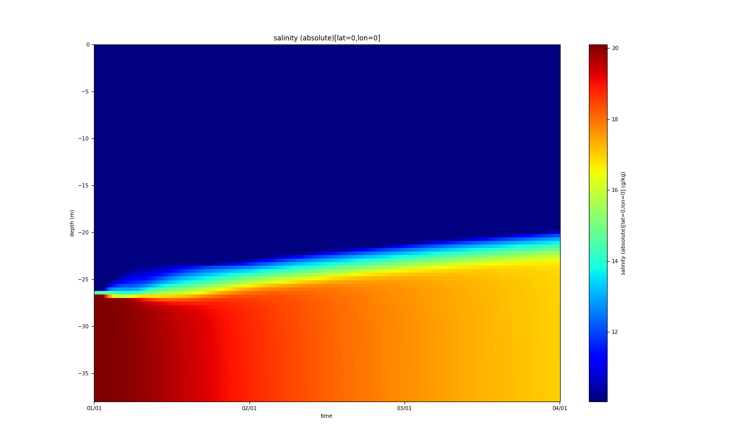
The plume is driven by a sloping bottom and density interface with the slope of tan(alpha_x)=tan(alpha_y)=-0.001, such that the vertically integrated transport is oriented towards the positive x-axis. The water depth is 38 m, and temperature and salinity are initialised such that a 12 m thick bottom boundary layer results with a density of about 8 kg/m3 higher than the ambient water above. Between plume and ambient water there is a linear transition layer of 0.5 m thickness. When initialised with zero velocity, the plume velocity in x-direction peaks after three days at about 0.5 m/s in the entrainment layer, while the velocity in y-direction in the entrainment layer has negative values of up to 0.3 m/s. This picture is consistent with the dynamics shown in Fig. 11 of Arneborg et al. (2007). During the three days of integration, the thickness of the bottom boundary layer increases by about 5 m.