Entrainment
The entrainment scenario is similar to the Couette scenario, except that the water column is now stably stratified by a vertically constant density gradient. Also in this scenario, the effect of Earth’s rotation is ignored. The entrainment scenario is ideally suited to benchmark model performance in stress-driven entrainment situations against available experiments (see Umlauf and Burchard, 2005). Various yaml files corresponding to different turbulence models can be found in the scenario directory to run and compare these different models. These include the k-epsilon model, the k-omega model of Umlauf et al. (2003), and the GLS (generic length scale) model described in Umlauf and Burchard (2003),). Note especially that now also the KPP implementation of CVMix is available in GOTM (Qing et al. 2021). Using gotm_cvmix.yaml in the scenario directory, this version of the KPP model can be run (don’t forget to run cmake with -DGOTM_USE_CVMIX=on before compiling the source code).
The results shown in the figure below illustrate that after the onset of the constant surface stress, a thin near-surface layer is accelerated (panel a), gradually entraining into the stratified, non-turbulent interior region. Shear-driven turbulence in this region is mirrored in the large turbulent diffusivities shown in panel (c), which generate a nearly well-mixed surface layer that is separated from the interior by a pycnocline of gradually increasing strength (panel b). The dashed lines show the entrainment model by Pollard et al. (1973) with the value for the bulk Richardson number suggested by Price (1979) for shear-driven entrainment into a linearly stratified fluid [see Eq. (53) in Umlauf and Burchard, 2005]. We now also provide the python script plot_entrainment.py used to generate the figure below
The numerical solution shown in the figure has been obtained with the k-ε model. Solutions for other two-equation models available in GOTM look similar.
Note that Pollard et al. (1973) also derived an entrainment model for the case with rotation. To compare this model to the GOTM solution, set “latitude: 45.0” in gotm.yaml, re-run the model, and uncomment lines 48-52 in plot_entrainment.py.
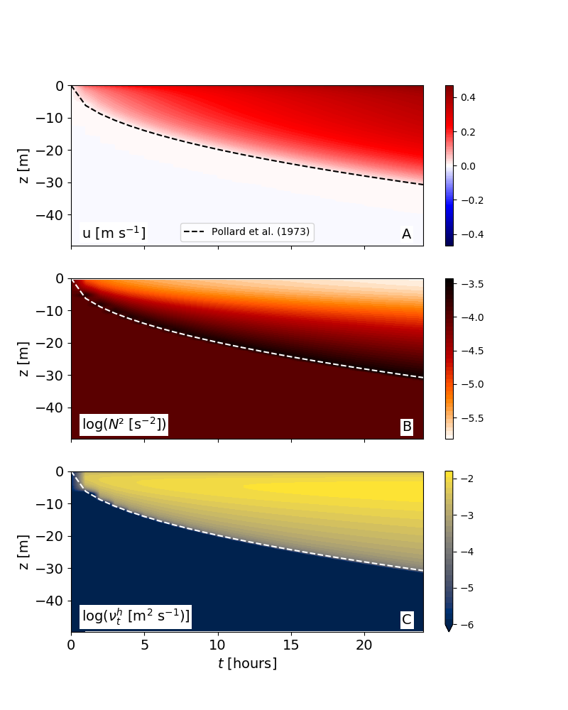
Evolution of (a) velocity, (b) buoyancy frequency squared, and (c) turbulent diffusivity. Dashed lines show the entrainment model of Pollard et al. (1973)