Coutte flow

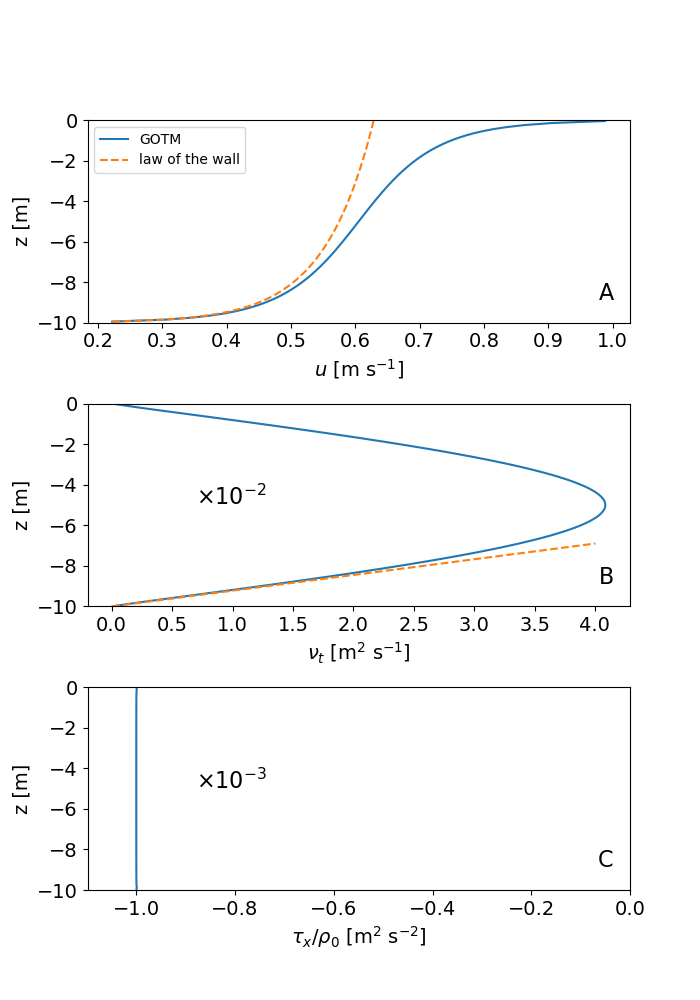
The Couette scenario is the most basic of all GOTM scenarios. It represents a shallow (10 m deep), unstratified layer of fluid above a flat bottom that is driven by a constant surface stress in the x-direction. Earth’s rotation is ignored. This flow is often referred to as a turbulent Couette flow. After the onset of the surface stress, a thin turbulent near-surface layer is generated that rapidly entrains into the non-turbulent deeper parts of the water column. The solution at the end of the simulation, when the problem has become fully stationary, is shown in the figure below. The velocity profile in panel (a) reveals the existence of two shear layers in the near-surface and near-bottom regions, respectively, that converge toward the analytical law-of-the-wall solutions (dashed red lines in the figure). The diffusivity profile in the turbulent Couette flow is nearly parabolic (panel b), and also converges to the linear law-of-the-wall solution near the boundaries. The Reynolds stress (or, likewise, the turbulent momentum flux) shown in panel (c) is perfectly constant throughout the water column, and corresponds exactly to the applied surface stress. This is easily understood from the fact that all momentum entering the water column at the surface has to leave it again at the bottom under stationary conditions. The solution shown in the figure has been obtained with the k-ε model. Solutions for other two-equation models like the k-ω model or the Mellor-Yamada model look similar (you can easily check this in the scenario directory by modifying the input file gotm.yaml). Technical details for this test case are described in the GOTM documentation. We now also provide the python script plot_couette.py used to generate the figure for this GOTM scenario (you will find this plotting script also in the case directory).